Lab 13

1. Provide the updated computer drawing for your individual RG setup.

Picture: Updated drawing

2. Explain your setup.

So a motor will be activated by Victoria's relay which will push a baseball down a ramp. The ramp at the bottom has a stopper and a pressure sensor and the ball will stop on the sensor activating the timer. The timer will count up to 4 then the power will go to the XOR gate and then through an opamp. The opamp boosts the voltage enough to switch over the relay and start the next part of the circuit. I had to take out the two displays because they didn't get enough voltage to illuminate so the voltage just goes to the motor. The motor flicks the flip gauge and sends voltage through the diode. The diode is connected to an opamp which boosts it to power a motor at the other end. The last motor will knock down a domino activating Daniels circuit.

3. Provide photos of the circuit and setup.

Picture: Current set up for updated RG

4. Provide at least 2 new videos of your setup in action, one being a failed attempt.

Video: The motor failing to push down the baseball

Video: Sensor activating the motor at the end of the circuit

5. What failures did you have? How did you overcome them?

One failure I ran across was the motor didn't push down the baseball, it was strong enough but if it wasn't aligned correctly it wouldn't go down. To fix this I adjusted the angle the motor was at to make it more inclined.

6. Group task: Explain your group RG setup.

Victoria's circuit will start, so first light will activate her circuit and cause a motor to spin. The motor is connected to a belt that will end up knocking a wheel down a ramp. The wheel will lead to another track that has a block stopping the next wheel. The first wheel knocks the block off releasing the last wheel to go down and knock off a block on a pressure sensor. The sensor is connected to a relay and allows power to switch over, leading to the start of my circuit. My motor is connected to the end of her relay and will knock the baseball down the ramp. The ball will stop at the end of the ramp and trigger a pressure sensor which will activate a timer. A counter is connected to the timer and once it reaches 4 the opamp would have increased the voltage enough to switch over the relay. The relay is connected to a motor that will hit the flip gauge generating a voltage. A diode is connected to the end of the flip gauge to only give positive voltage which will go through an opamp. The opamp boosts the voltage enough to power a motor that will knock down some domions leading to Daniel's circuit.

7. Group task: Video of a test run of your group RG.

Video: Group RG Explained

Video: The Transition

Video: Group RG Failed Attempt

Victoria's Part

1. Provide the updated computer drawing for your individual RG setup.

Figure: Updated Circuit Schematic

2. Explain your setup.

Removing covering from the photoresistor allows enough current to flow through an opamp to trigger a relay. this relay then powers a motor which turns a conveyor belt. the conveyor belt then knocks a dominoe into a cart which will roll down a ramp. at the bottom of this ramp, there is a loose blockage which will be pushed off by the first cart. with the blockage gone, a second cart will fall down a second ramp. This cart will then remove an object from a pressure sensor. this pressure sensor is connected to a voltage source and opamp so that when the pressure is removed, the sensor would trigger a switch in the relay. When the relay switches, the output that turns off will turn of the other relay because it is connected to the first relay's upper bound input. The other output of the second relay will then spin a motor which triggers James' circuit.

3. Provide photos of the circuit and setup.

Image: New Circuit Setup

Image: Mechanical Setup

4. Provide at least 2 new videos of your setup in action, one being a failed attempt.

Video: My Rube Goldberg Fail

Video: My Rube Goldberg Success 

5. What failures did you have? How did you overcome them?
A major issue I experienced was the inconsistency of the pressure sensor; what worked repeatedly well last week, almost never worked this week. To combat this, I tried adjusting connections and changing the gain on the opamp to accommodate the new values. Also, I had a problem earlier with my motor running out of control after it served its function. this is now minimized by the fact that the first relay's input is connected to the second relay's output, so when voltage goes to James' setup, it no longer goes to mine.

Lab 12

James Tompkins Part

1. Provide the computer drawing for your individual RG setup.

Picture: Computer drawing of circuit
2. Explain your setup.

 At the end of Victoria's cricuit a pressure sensor will be triggered which will allow a motor to run, releasing a ball on a ramp. The ball will travel down and land on my pressure sensor that is connected to the 555 timer and the 74192, which will then send current to the 7447 and a counter, once the counter reaches a certain number, the gate will be activated and lead to a opamp connected to a relay. On the other end of the relay, once the flip is switched, are 2 displays spelling out "HI" and then another wire connecting the motor. The motor will spin and flick the flick gauge which will then go through a diode and capacitor to give off voltage for the next circuit.

3. Provide photos of the circuit and setup.

Picture: James circuit set up

4. Provide at least 2 videos of your setup in action (parts or whole), at least one being a failed attempt.

Video 1: motor and flip gauge generating voltage

Video 2: motor and flip gauge failing to connect

Video 3: activation of the circuit

5. What failures did you have? How did you overcome them?

A error I had was the motor would not always connect to the gauge, so I extended it so it hits every time now.

Victoria Heini Part:

1. Provide the computer drawing for your individual RG setup.

Figure 1: Circuit Schematic:

Figure 2: Mechanical Component

2. Explain your setup.
The circuit is triggered by a photoresistor. When the resistor is uncovered, the voltage passing through it is amplified to about 8 volts so that the relay is triggered. The triggered relay then spins the motor, which is connected to the gears of the conveyor belt which is the component in the upper left hand of Figure 2. This then causes a domino to be pushed into a set of wheels at the top  of a ramp. this contraption roles downward until it pushes a block of of another ramp. With this obstacle gone, another set of wheels is allowed to roll down a second ramp so that it knocks over a block standing on a pressure sensor. The change in pressure on the pressure sensor, with the addition of a second operation amplifier, triggers a second relay.

3. Provide photos of the circuit and setup.

Image: Circuit Layout

Image: Entire Set-up

Image: Conveyor Belt

Image: Ram 2 with Blockage

4. Provide at least 2 videos of your setup in action (parts or whole), at least one being a failed attempt.

Video: Failed Attempt

Video: Some Minor Success

5. What failures did you have? How did you overcome them?

Initially, the pressure sensor was going to be incorporated so that other items would fall on it causing a change in pressure that could supply a voltage to another component. This proved to be difficult because making something consistently fall in the same way is more complicated than simply making something fall consistently. After fixing this, there was still a problem getting the mechanical parts to move as the should; ie., the dominoes on the conveyor belt did not cause the cart to roll, and the second cart did not successfully more the mass on the pressure sensor. The former was solved by making the cart a larger and closer target, and the second was solved by making the second cart heavier.

Lab 11

Blog sheet Week 11: Strain Gauges

Part A: Strain Gauges:

Strain gauges are used to measure the strain or stress levels on the materials. Alternatively, pressure on the strain gauge causes a generated voltage and it can be used as an energy harvester. You will be given either the flapping or tapping type gauge. When you test the circle buzzer type gauge, you will lay it flat on the table and tap on it. If it is the long rectangle one, you will flap the piece to generate voltage.

1. Connect the oscilloscope probes to the strain gauge. Record the peak voltage values (positive and negative) by flipping/tapping the gauge with low and high pressure. Make sure to set the oscilloscope horizontal and vertical scales appropriately so you can read the values. DO NOT USE the measure tool of the oscilloscope. Adjust your oscilloscope so you can read the values from the screen. Fill out Table 1 and provide photos of the oscilloscope.

Flipping Strength	Min Voltage (V)	Max Voltage (V)
Low	-2	4.4
High	-27.2	14.4

Tapping Strenght	Min Voltage (V)	Max Voltage (V)
Low	-1	1.8
High	-4	24.8

Table 1: Strain gauge characteristics

Picture: Low tapping on the sensor

Picture: High tapping on the sensor

2. Press the “Single” button below the Autoscale button on the oscilloscope. This mode will allow you to capture a single change at the output. Adjust your time and amplitude scales so you have the best resolution for your signal when you flip/tap your strain gauge. Provide a photo of the oscilloscope graph.

Picture: Single Wave of Tapping Gauge

Picture: Single Wave of Flicking Gauge

Part B: Half-Wave Rectifiers

1. Construct the following half-wave rectifier. Measure the input and the output using the oscilloscope and provide a snapshot of the outputs.

Picture: Oscilloscope reading of the half-wave rectifier

2. Calculate the effective voltage of the input and output and compare the values with the measured ones by completing the following table.

Effective Rms	Calculated	Measured
Input	7.07	7.25
Output	3.54	3.63

3. Explain how you calculated the rms values. Do calculated and measured values match?

The rms value of the input is calculated by by dividing the peak to peak input voltage by the square root of 2 as a simplification of the following integral for a  sin wave:

Equation: RMS Equation as Found on Wikipedia


Because an integral describes the area under a curve, it is clear that the area of the output wave should be half of that of the input. So the simplified integral calculation for the output becomes the input peak to peak voltage divided by the quantity of 2 times the square root of 2.

With this calculation and the measurements at the output, there appears to be an apparent consistency within a reasonable margin of error.

4. Construct the following circuit and record the output voltage using both DMM and the oscilloscope.

	Oscilloscope	DMM
Output Voltage (P2P) (V)	9.6	2.725
Out Put Voltage (Mean) (V)	.225	3.9

5. Replace the 1 µF capacitor with 100 µF and repeat the previous step. What has changed?

	Oscilloscope	DMM
Output Voltage (P2P) (V)	.596	.125
Out Put Voltage (Mean) (V)	Jumps from 2 to-4	6.44

With a higher capacitance, the range of the oscillations was significantly decreased, but the mean of the output voltage significantly increased presumably because the stronger capacitor stored more voltage. It also became difficult to get a consistent reading particularly for the output voltage mean. we hypothesize that this might be caused by the capacitor's function of storing and releasing voltage.

Part C: Energy Harvesters
1. Construct the half-wave rectifier circuit without the resistor but with the 1 µF capacitor. Instead of the function generator, use the strain gauge. Discharge the capacitor every time you start a new measurement. Flip/tap your strain gauge and observe the output voltage. Fill out the table below:

	Time (s)	Output (mV)
1 Flip per Second	10	26
1 Flip per Second	20	102
1 Flip per Second	30	61
4 Flip per Second	10	103
4 Flip per Second	20	346
4 Flip per Second	30	603

	Time (s)	Output (mV)
1 Tap per Second	10	375
1 Tap per Second	20	430
1 Tap per Second	30	350
4 Tap per Second	10	2800
4 Tap per Second	20	2300
4 Tap per Second	30	3000

2. Briefly explain your results.

We noticed when doing the flips and taps per second, that if you hit it harder at first then not as hard the time after it started to decrease even though it was still being hit. After noticing this, it helped reason why some of our numbers ended up seeming off in perspective to the values before.

3. If we do not use the diode in the circuit (i.e. using only strain gauge to charge the capacitor), what would you observe at the output? Why?

There is little to no change in the graph, because the diode only allows the positive part of the wave to pass through and without it the wave ends up canceling itself out.This is because if only a positive input is allowed to effect the output, it can continue to increase the voltage, but if the negative portion of the wave passes through as well the output voltage would have a tendency to make a small increase followed by a small decrease and repeating this in a cyclical pattern resulting in no net gain in voltage.

4. Write a MATLAB code to plot the date in table of Part C1.

Flick Gauge MATLAB Code:

Flick plot:
x=[10 20 30];
y1=[26 102 61];
y2=[103 346 603];
y3=[375 430 350];
y4=[2800 2300 3000];
plot(x,y1,'o-',x,y2,'s-')
xlabel('Duration (s)')
ylabel('Output Voltage (mV)')
legend('1 Flick per second','4 Flicks per second')

Graph: Flick Gauge Voltages After Different Intervals of Consistent Flicking

Tap Guage MATLAB Code:

Tap plot:
plot(x,y3,'o-',x,y4,'s-')
xlabel('Duration (s)')
ylabel('Output Voltage (mV)')
legend('1 Tap per second','4 Taps per second')

Graph: Tap Gauge Voltages After Different Intervals of Consistent Tapping

Lab 10

In this week’s lab, you will collect more data on low pass and high pass filters and “process” them using MATLAB.
PART A: MATLAB practice.

1. Open MATLAB. Open the editor and copy paste the following code. Name your code as FirstCode.m
Save the resulting plot as a JPEG image and put it here.
clear all;
close all;
x = [1 2 3 4 5];
y = 2.^x;
plot(x, y, 'LineWidth', 6)
xlabel('Numbers', 'FontSize', 12)
ylabel('Results', 'FontSize', 12)


2. What does clear all do?

Clear all simply clears the command window.

3. What does close all do?

Close all clears the command window and closes all MATLAB figures and graphs etc.

4. In the command line, type x and press enter. This is a matrix. How many rows and columns are there in the matrix?

There is one row and 5 columns in the matrix x.
x =
     1     2     3     4     5

5. Why is there a semicolon at the end of the line of x and y?
The semicolon keeps the x and y from being displayed in the command window when the code is ran.

6. Remove the dot on the y = 2.^x; line and execute the code again. What does the error message mean?
It means that with out the period multiple values of x and y cannot be calculated.

7. How does the LineWidth affect the plot? Explain.
This is how thick the line on the plot is going to be.

8. Type help plot on the command line and study the options for plot command. Provide how you would change the line for plot command to obtain the following figure (Hint: Like ‘LineWidth’, there is another property called ‘MarkerSize’)

x = [1 2 3 4 5];

y = 2.^x;

plot(x,y,'r-o','Linewidth',5,'markersize',15)
xlabel('Numbers', 'FontSize', 12)

ylabel('Results', 'FontSize', 12)

9. What happens if you change the line for x to x = [1; 2; 3; 4; 5]; ? Explain.

For this code, the array for "x" becomes a vertical one instead of a horizontal one; ie., there is one column with 5 rows instead of 5 columns with one row. The corresponding output is shown below:

x =

     1
     2
     3
     4
     5
However, this change in the x array does not change the values for "y" and thus the plot remains the same.

10. Provide the code for the following figure. You need to figure out the function for y. Notice there are grids on the plot.

plot(x,y,'k:s','Linewidth',5,'markersize',15)
xlabel('Numbers', 'FontSize', 12)

ylabel('Results', 'FontSize', 12)
x
GridLineStyle = '--'
grid on


11. Degree vs. radian in MATLAB:

a. Calculate sinus of 30 degrees using a calculator or internet.
The calculated value of sin 30 is .5.

b. Type sin(30) in the command line of the MATLAB. Why is this number different? (Hint: MATLAB treats angles as radians).
MATLAB uses radians as a default measurement and if the user wants degrees they just have to change the code a bit. Below, the code and the output are displayed for "sin(30)."
>> sin(30)

ans =

   -0.9880

c. How can you modify sin(30) so we get the correct number?

Using just "sin" will be accurate for values in radians, but to get values for degrees, "sind" can be used instead. The MATLAB input and output are displayed here:
>> sind(30)

ans =

    0.5000

12. Plot y = 10 sin (100 t) using Matlab with two different resolutions on the same plot: 10 points per period and 1000 points per period. The plot needs to show only two periods. Commands you might need to use are linspace, plot, hold on, legend, xlabel, and ylabel. Provide your code and resulting figure. The output figure should look like the following:

Graph: Sinusoidal curve of how the coarse would normally appear

To obtain this graph, the following code was entered into MATLAB:

t=linspace(0,4*pi/100,10);
y=10.*sin(100.*t);
plot(t,y,'r-o')
hold on
t2=linspace(0,4*pi/100,1000);
y2=10.*sin(100.*t2);
plot(t2,y2,'k')
xlabel('Time (s)')
ylabel('y function')
legend('Coarse','Fine')

Note that the upper value of the linspace command for the two different t values is 4*pi/100. this is because the graph is of the first 2 periods and the period of a sinusoidal function is 2pi/b where "b" is the coeffecient of "t" in the sin function (y=Asin(bt)). So, to show two periods, 2pi/ b was multiplied by 2 to get 4pi/100.

13. Explain what is changed in the following plot comparing to the previous one.

Graph: Function with a maximum value of 5, and what it would normally look like

So for the updated graph, the fine value has a set maximum of 5 now, as opposed to the original function that had a maximum value of 10. Because there are values that would normally be about the 5, the new graph just flattens out at the maximum.

14. The command find was used to create this code. Study the use of find (help find) and try to replicate the plot above. Provide your code.

t=linspace(0,4*pi/100,10);
y=10.*sin(100.*t);
plot(t,y,'r-o')
hold on
t2=linspace(0,4*pi/100,1000);
y2=10.*sin(100.*t2);
%plot(t2,y2,'k')
xlabel('Time (s)')
ylabel('y function')
legend('Coarse','Fine')
I=find(y2<5);
t3= t2(I);
y3= y2(I);
plot(t3,y3,'k')

To obtain the graph from 13, the above code was entered. the "find" code finds the indices of the values of a vector that are above or below a certain value. For this function, we used "find" to find the values for y2 that were less than 5, where y2 was the smooth function for 10sin(100t). With these indices found, we called these values to the new matrices of t3 for time and y3 for the y values of the function. Then we plotted y3 with respect to t3 to get the graph displayed above.

PART B: Filters and MATLAB
1. Build a low pass filter using a resistor and capacitor in which the cut off frequency is 1 kHz.
Observe the output signal using the oscilloscope. Collect several data points particularly around the cut off frequency. Provide your data in a table.

Frequency (Hz)	Output rms Voltage (V)
10	0.838
50	0.847
100	0.849
200	0.838
300	0.820
400	0.797
500	0.768
600	0.737
700	0.709
800	0.680
850	0.668
900	0.648
950	0.637
1000	0.625
1050	0.607
1100	0.599
1150	0.583
1200	0.573
1300	0.545
1400	0.516
1500	0.493

Table: Low pass filter frequency and resulting output voltage

*Input is 1 V peak to peak, or 0.707 rms V.

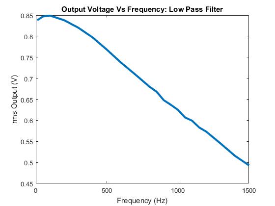
2. Plot your data using MATLAB. Make sure to use proper labels for the plot and make your plot line and fonts readable. Provide your code and the plot.

MATLAB Code:

F=[10 50 100 200 300 400 500 600 700 800 850 900 950 1000 1050 1100 1150 ...
    1200 1300 1400 1500]
Vout=[.838 .847 .849 .838 .820 .797 0.768 .737 .709 .680 .668 .648 .637 ...
    .625 .607 .599 .583 .573 .545 .516 .493]
plot(F,Vout,'LineWidth', 3)
xlabel('Frequency (Hz)')
ylabel('rms Output (V)')
title ('Output Voltage Vs Frequency: Low Pass Filter')












Graph: Low pass filter and resulting output voltage

3. Calculate the cut off frequency using MATLAB. find command will be used. Provide your code.

MATLAB Code:

F=[10 50 100 200 300 400 500 600 700 800 850 900 950 1000 1050 1100 1150 ...
    1200 1300 1400 1500];
Vout=[.838 .847 .849 .838 .820 .797 0.768 .737 .709 .680 .668 .648 .637 ...
    .625 .607 .599 .583 .573 .545 .516 .493];
plot(F,Vout,'LineWidth', 3)
xlabel('Frequency (Hz)')
ylabel('rms Output (V)')
title ('Output Voltage Vs Frequency: Low Pass Filter')
hold on
c=find(Vout<.707*.838);
d=c(1);
CutoffFrequency=F(d)

MATLAB Output:
CutoffFrequency =

        1150

4. Put a horizontal dashed line on the previous plot that passes through the cutoff frequency.

Graph: Low pass filter frequency with respect to voltage

5. Repeat 1-3 by modifying the circuit to a high pass filter.

      5.1. 

Frequency (Hz)	Output rms Voltage (V)
10	0.030
50	0.048
100	0.072
200	0.163
300	0.235
400	0.301
500	0.369
600	0.423
700	0.467
800	0.516
850	0.532
900	0.549
950	0.568
1000	0.582
1050	0.596
1100	0.610
1150	0.622
1200	0.634
1300	0.655
1400	0.678
1500	0.689

Table: High pass filter frequency and the resulting output voltage

      5.2.

MATLAB Code:

F=[10 50 100 200 300 400 500 600 700 800 850 900 950 1000 1050 1100 1150 ...

    1200 1300 1400 1500];

Vout=[0.030 .048 .072 .162 .235 .301 .369 .423 .467 .516 .532 .544 .568 ...

    .582 .596 .610 .622 .634 .655 .678 .689];

plot(F,Vout,'LineWidth', 3)

xlabel('Frequency (Hz)')

ylabel('rms Output (V)')

title ('Output Voltage Vs Frequency: High Pass Filter')

Graph: High pass filter frequency with respect to voltage

    5.3  Calculate the cut off frequency using MATLAB. find command will be used. 

F=[10 50 100 200 300 400 500 600 700 800 850 900 950 1000 1050 1100 1150 ...

    1200 1300 1400 1500];

Vout=[.030 .048 .072 .162 .235 .301 .369 .423 .467 .516 .532 .544 .568 ...

    .582 .596 .610 .622 .634 .655 .678 .689];

plot(F,Vout,'LineWidth', 3);

xlabel('Frequency (Hz)');

ylabel('rms Output (V)');

title ('Output Voltage Vs Frequency: Low Pass Filter');

x=find(Vout>.549);

c=F(s);

cutoff= min(c)

cutoff =

   950